Introduction to Hamiltonian

(Not technically correct, but still funny.)
Image source

Introduction

\[i\hbar\frac{\partial}{\partial t}\ket{\psi} = \mathcal{H}\ket{\psi}\]

Do you remember this equation? It’s the Schrödinger’s equation, which we first encountered in the beginning of this series. Back then, we mentioned that $\mathcal{H}$ is some quantum operator acting on the quantum state $\ket{\psi}$, but we skipped over its meaning.

In this article, we’ll unpack the true identity of $\mathcal{H}$, which is called Hamiltonian.

Energy of a System

Hamiltonian is closely related to the energy of a physical system. To build intuition, let’s start with a classical example: imagine a ball with mass $m$, moving at speed $v$ and located at height $h$.

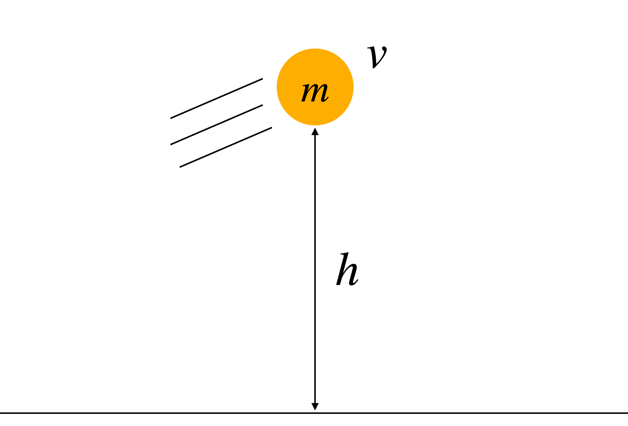
In classical mechanics, the total energy of the system is the sum of its kinetic and potential energy.

• Kinetic energy:

  \[\frac{1}{2}mv^2\]

• Potential energy (due to gravitational acceleration $g$):

  \[mgh\]

Thus, the total energy of the system is:

\[E = \frac{1}{2}mv^2 + mgh.\]

For example, throwing a $m=1\text{ kg}$ ball at speed $v=10\text{ m/s}$ from a height $h = 5 \text{ m}$ gives (assume $g = 10 \text{ m/s}^2$):

\[E = \frac{1}{2}(1)(10)^2 + (1)(10)(5) = 50 + 50 = 100 \text{ J}.\]

Hamiltonian as a Function

From a programmer’s point of view, this energy value looks like a hard-coded constant ($100\text{ J}$). But since the ball’s position and speed constantly change, we’d typically write a function that computes energy from the system state:

def calculate_energy(state):
    m = 1  # kg
    g = 10  # m/s^2
    h = state['height']  # m
    v = state['speed']  # m/s
    return (1/2) * m * v**2 + m * g * h

This is essentially what the Hamiltonian does: it computes the energy of a system from its state.

In classical mechanics, the Hamiltonian is just like a formula:

\[\mathcal{H}(h, v) = \frac{1}{2}mv^2 + mgh.\]

In quantum mechanics, however, it becomes an operator—a matrix-like object that acts on quantum states $\ket{\psi}$ in a Hilbert space.

To compute the energy of a quantum state, we use the expression:

\[\bra{\psi}\mathcal{H}\ket{\psi} = E.\]

This gives the expectation value of the system’s energy if it is in state $\ket{\psi}$.

Energy of a Quantum System

So why is $\bra{\psi}\mathcal{H}\ket{\psi}$ only an expectation value? Because in quantum mechanics, energy is quantized.

That is, a system can only have certain discrete energy levels, not any arbitrary value. For example, the electron in a hydrogen atom can only occupy energy levels labeled $n=1, 2, 3, \ldots$:

Image source

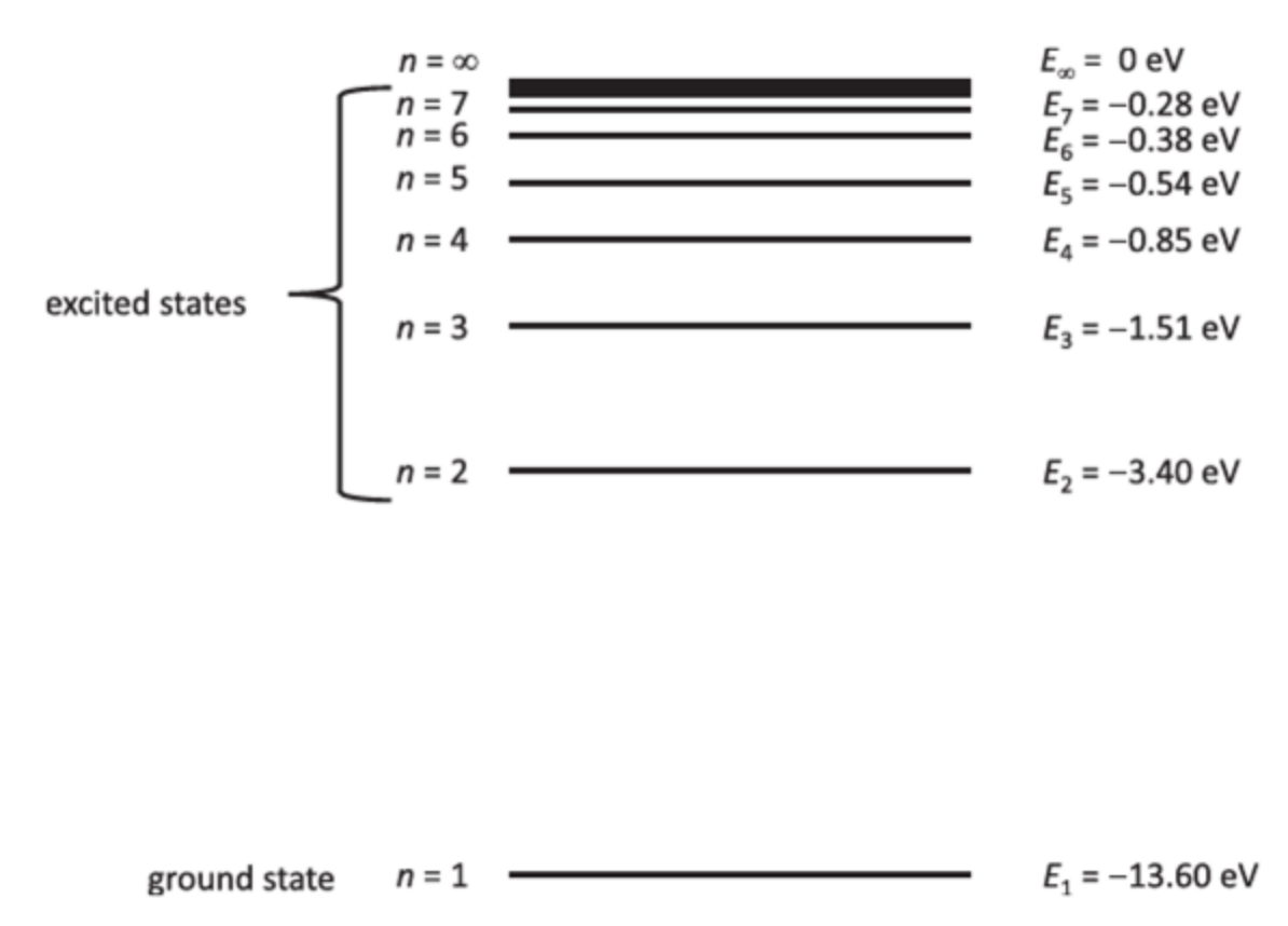
Each energy level corresponds to a different state of the system. For the hydrogen atom example above, we can call the state of the energy level $n$ as $\ket{\phi_n}$.

The Hamiltonian $\mathcal{H}$ of the system determines these energy levels and the corresponding states. More precisely, these are defined by:

\[\mathcal{H}\ket{\phi_n} = E_n\ket{\phi_n},\]

where $\ket{\phi_n}$ is an eigenstate of the Hamiltonian and $E_n$ is its corresponding eigenvalue.

One of the beautiful mathematical results in quantum mechanics is that these eigenstates from an orthonormal basis of the Hilbert space (just like $\ket{0}$ and $\ket{1}$ in the qubit space). That means any quantum state $\ket{\psi}$ can be expressed as a superposition of the energy eigenstates:

\[\ket{\psi} = \sum_n c_n\ket{\phi_n},\]

Now it becomes clear why $\bra{\psi}\mathcal{H}\ket{\psi}$ gives only the expected energy: the state may be a mix of different energy eigenstates, each with its own energy. Let’s look at a simple example.

Suppose the system is in a uniform superposition of just two energy eigenstates:

\[\ket{\psi} = \frac{1}{\sqrt{2}}(\ket{\phi_0} + \ket{\phi_1}).\]

Then the expectation value of the energy is:

\[\begin{align*} \bra{\psi}\mathcal{H}\ket{\psi} &=\frac{1}{2}(\bra{\phi_0}+\bra{\phi_1})\mathcal{H}(\ket{\phi_0}+\ket{\phi_1})\\ &=\frac{1}{2}(\bra{\phi_0}+\bra{\phi_1})(\mathcal{H}\ket{\phi_0}+\mathcal{H}\ket{\phi_1})\\ &=\frac{1}{2}(\bra{\phi_0}+\bra{\phi_1})(E_0\ket{\phi_0}+E_1\ket{\phi_1})\\ &=\frac{1}{2}(E_0\braket{\phi_0}{\phi_0}+E_1\braket{\phi_1}{\phi_1})\\ &=\frac{1}{2}(E_0+E_1), \end{align*}\]

This is simply the average of the two energy levels $E_0$ and $E_1$. The simplification works because the eigenstates are orthonormal:

\[\braket{\phi_0}{\phi_0}=\braket{\phi_1}{\phi_1}=1,\quad \braket{\phi_0}{\phi_1}=\braket{\phi_1}{\phi_0}=0.\]

But here’s the important part: if you measure the energy of the system in state $\ket{\psi}=\frac{1}{\sqrt{2}}(\ket{\phi_0}+\ket{\phi_1})$, you won’t get the average. You’ll get either $E_0$ or $E_1$ with 50% probability. After the measurement, the system collapses into the corresponding eigenstate $\ket{\phi_0}$ or $\ket{\phi_1}$, and is no longer in a superposition.

which is the average of the energies of the two eigenstates $\ket{\phi_0}$ and $\ket{\phi_1}$, as expected. Note that $\braket{\phi_0}{\phi_0}=\braket{\phi_1}{\phi_1}=1$ and $\braket{\phi_0}{\phi_1}=\braket{\phi_1}{\phi_0}=0$, since $\ket{\phi_n}$ forms an orthonormal basis of the Hilbert space.

If we measure the energy of the system of this state $\ket{\psi}=\frac{1}{\sqrt{2}}(\ket{\phi_0}+\ket{\phi_1})$, we will get either $E_0$ or $E_1$ with 50% chance, not the average of the two energies. This is because the measurement collapses the state of the system to one of the eigenstates $\ket{\phi_0}$ or $\ket{\phi_1}$, which means that the system is no longer in a superposition of the two states.

Hamiltonian the Almighty

The Hamiltonian $\mathcal{H}$ is packed with information about the system. It gives us:

• All possible energy levels and their corresponding eigenstates,

• And how the system evolves over time, via the Schrödinger’s equation:

  \[i\hbar\frac{\partial}{\partial t}\ket{\psi} = \mathcal{H}\ket{\psi}\]

Here, the left-hand side represents how the state changes with time, and the right-hand side is the Hamiltonian acting on the current state.

Thanks to the Hamiltonian, physicists can understand and predict the system’s behavior—not by drawing balls, springs, or arrows, but by working directly with equations.